Introduction to Data Structures & Algorithms
Table of contents
- Data Structures and Algorithms:
- Some other Important terminologies:
- Memory Layout of C Programs:
- Time Complexity and Big O Notation
- Asymptotic Notations: Big O, Big Omega and Big Theta
- Best Case, Worst Case and Average Case Analysis of an Algorithm
- Arrays and Abstract Data Type in Data Structure
- Linear Vs Binary Search + Code in C Language
Data Structures and Algorithms:
Let's clear up our basics with these terms before deep diving into DSA. Data Structures and Algorithms are two different things.
Data Structures – These are like the ingredients you need to build efficient algorithms. These are the ways to arrange data so that they (data items) can be used efficiently in the main memory. Examples: Array, Stack, Linked List, and many more. You don't need to worry about these names. These topics will be covered in detail in the upcoming tutorials.
Algorithms – Sequence of steps performed on the data using efficient data structures to solve a given problem, be it a basic or real-life-based one. Examples include: sorting an array.
Some other Important terminologies:
Database – Collection of information in permanent storage for faster retrieval and updation. Examples are MySql, MongoDB, etc.
Data warehouse – Management of huge data of legacy data( the data we keep at a different place from our fresh data in the database to make the process of retrieval and updation fast) for better analysis.
Big data – Analysis of too large or complex data, which cannot be dealt with the traditional data processing applications.
Memory Layout of C Programs:
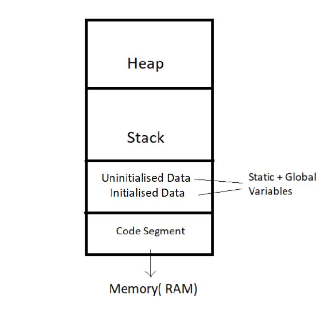
When the program starts, its code gets copied to the main memory.
The stack holds the memory occupied by functions. It stores the activation records of the functions used in the program. And erases them as they get executed.
The heap contains the data which is requested by the program as dynamic memory using pointers.
Initialized and uninitialized data segments hold initialized and uninitialized global variables, respectively.
Take a look at the below diagram for a better understanding:
Time Complexity and Big O Notation
What is Time Complexity?
Time Complexity is the study of the efficiency of algorithms. It tells us how much time is taken by an algorithm to process a given input. Let's understand this concept with the help of an example:
Consider two developers Divyansh and Adarsh , who created an algorithm to sort ‘n’ numbers independently. When they made the program run for some input size n, the following results were recorded:
| No. of elements (n) | Time Taken By Divyansh’s Algo | Time Taken By Adarsh’s Algo |
| 10 elements | 80 ms | 102 ms |
| 70 elements | 100 ms | 114 ms |
| 110 elements | 150 ms | 121 ms |
| 1000 elements | 2s | 800 ms |
We can see that at first, Divyansh’s algorithm worked well with smaller inputs; however, as we increase the number of elements, Adarsh’s algorithm performs much better.
Calculating Order in terms of Input Size:
In order to calculate the order(time complexity), the most impactful term containing n is taken into account (Here n refers to Size of input). And the rest of the smaller terms are ignored.
Let us assume the following formula for the algorithms in terms of input size n:
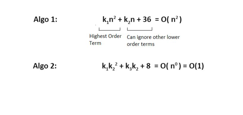
Here, we ignored the smaller terms in algo 1 and carried the most impactful term, which was the square of the input size. Hence the time complexity became n^2. The second algorithm followed just a constant time complexity.
What is a Big O?
Putting it simply, big O stands for ‘order of’ in our industry, but this is pretty different from the mathematical definition of the big O. Big O in mathematics stands for all those complexities our program runs in. But in industry, we are asked the minimum of them. So this was a subtle difference.
Visualizing Big O:
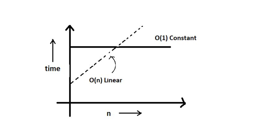
If we were to plot O(1) and O(n) on a graph, they would look something like this:

Asymptotic Notations: Big O, Big Omega and Big Theta
Asymptotic notation gives us an idea about how good a given algorithm is compared to some other algorithm.
Now let's look at the mathematical definition of 'order of.' Primarily there are three types of widely used asymptotic notations.
Big oh notation ( O )
Big omega notation ( Ω )
Big theta notation ( θ ) – Widely used one
Big oh notation ( O ):
Big oh notation is used to describe an asymptotic upper bound.
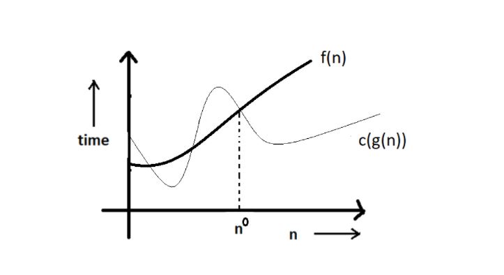
Mathematically, if f(n) describes the running time of an algorithm; f(n) is O(g(n)) if and only if there exist positive constants c and n° such that:
0 <= f(n) <= c g(n) for all n >= n**0
Here, n is the input size, and g(n) is any complexity function, for, e.g. n, n2, etc. (It is used to give upper bound on a function)
If a function is O(n), it is automatically O(n2) as well! Because it satisfies the equation given above.
Graphic example for Big oh ( O ):

Big Omega Notation ( Ω ):
Just like O notation provides an asymptotic upper bound, Ω notation provides an asymptotic lower bound.
Let f(n) define the running time of an algorithm; f(n) is said to be Ω (g(n)) if and only if there exist positive constants c and n° such that:
0 <= c g(n) <= f(n) for all n >= n**0It is used to give the lower bound on a function.
If a function is Ω (n2) it is automatically Ω (n) as well since it satisfies the above equation.
Graphic example for Big Omega (Ω):
Big theta notation ( θ ):
Let f(n) define the running time of an algorithm.
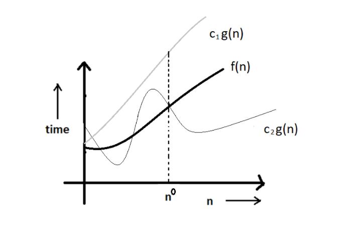
F(n) is said to be θ (g(n)) if f(n) is O (g(n)) and f(x) is Ω (g(n)) both.
0 <= c2 g(n) <= f(n) <= c1 g(n) for all n > n**0
The equation simply means that there exist positive constants c1 and c2 such that f(n) is sandwiched between c2 g(n) and c1 g(n).
Graphic example of Big theta ( θ ):
Best Case, Worst Case and Average Case Analysis of an Algorithm
Analysis of a search algorithm:
Consider an array that is sorted in increasing order.
7 | 8 | 29 | 31 |
We have to search a given number in this array and report whether it’s present in the array or not. In this case, we have two algorithms, and we will be interested in analyzing their performance separately.
Algorithm 1 – Start from the first element until an element greater than or equal to the number to be searched is found.
Algorithm 2 – Check whether the first or the last element is equal to the number. If not, find the number between these two elements (center of the array); if the center element is greater than the number to be searched, repeat the process for the first half else, repeat for the second half until the number is found. And this way, keep dividing your search space, making it faster to search.
Analyzing Algorithm 1: (Linear Search)
- We might get lucky enough to find our element to be the first element of the array. Therefore, we only made one comparison which is obviously constant for any size of the array.
- Best case complexity = O(1)
- If we are not that fortunate, the element we are searching for might be the last one. Therefore, our program made ‘n’ comparisons.
- Worst-case complexity = O(n)
For calculating the average case time, we sum the list of all the possible case’s runtime and divide it with the total number of cases. Here, we found it to be just O(n). (Sometimes, calculation of average-case time gets very complicated.)
Analyzing Algorithm 2: (Binary Search)
- If we get really lucky, the first element will be the only element that gets compared. Hence, a constant time.
- Best case complexity = O(1)
If we get unlucky, we will have to keep dividing the array into halves until we get a single element. (that is, the array gets finished)
Hence the time taken : n + n/2 +n/4 + . . . . . . . . . . + 1 = log n with base 2
Worst-case complexity = O(log n)
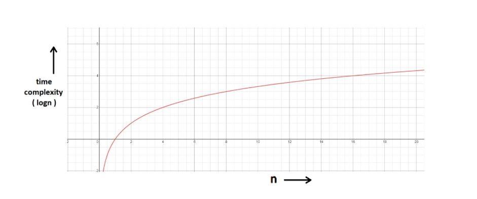
log(n)
Logn refers to how many times I need to divide n units until they can no longer be divided (into halves).
log8 = 3 ⇒ 8/2 + 4/2 + 2/2 → Can’t break anymore.
log4 = 2 ⇒ 4/2 + 2/2 → Can’t break anymore.
You can refer to the graph below, and you will find how slowly the time complexity (Y-axis) increases when we increase the input n (X-axis).
Space Complexity:
Time is not the only thing we worry about while analyzing algorithms. Space is equally important.
Creating an array of size n (size of the input) → O (n) Space
If a function calls itself recursively n times, its space complexity is O (n).
Arrays and Abstract Data Type in Data Structure
Abstract Data Types and Arrays:
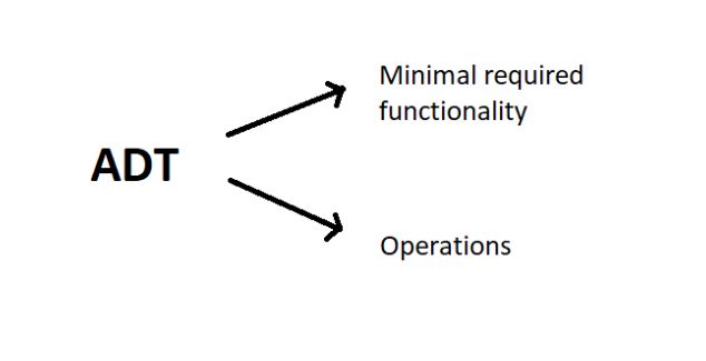
ADTs or abstract data types are the ways of classifying data structures by providing a minimal expected interface and some set of methods. It is very similar to when we make a blueprint before actually getting into doing some job, be it constructing a computer or a building. The blueprint comprises all the minimum required logistics and the roadmap to pursuing the job.
Array - ADT
An array ADT holds the collection of given elements (can be int, float, custom) accessible by their index.
1. Minimal required functionality:
We have two basic functionalities of an array, a get function to retrieve the element at index i and a set function to assign an element to some index in the array.
get (i) – get element i
set (i, num) – set element i to num.
2. Operations:-
We can have a whole lot of different operations on the array we created, but we’ll limit ourselves to some basic ones.
Max()
Min()
Search ( num )
Insert ( i, num )
Append (x)
Let the below-illustrated array be an example of what we are talking about.
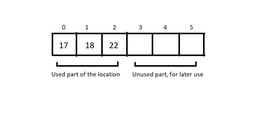
Here, the total_size returns 6, and the used_size returns 3.
Linear Vs Binary Search + Code in C Language
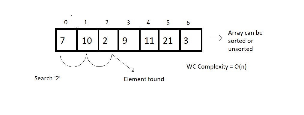
Linear Search:
This search method searches for an element by visiting all the elements sequentially until the element is found or the array finishes. It follows the array traversal method.
Binary Search:
This search method searches for an element by breaking the search space into half each time it finds the wrong element. This method is limited to a sorted array. The search continues towards either side of the mid, based on whether the element to be searched is lesser or greater than the mid element of the current search space.
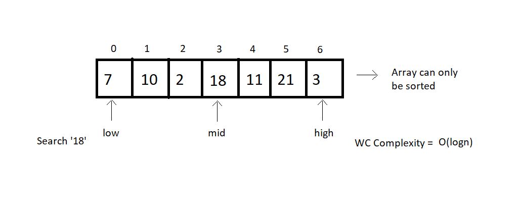
Comparison between both the search methods based on their choice of arrays, operations, and worst-case complexities.
| | Linear Search | Binary Search | | --- | --- | --- | | 1. | Works on both sorted and unsorted arrays | Works only on sorted arrays | | 2. | Equality operations | Inequality operations | | 3. | O(n) WC Complexity | O(log n) WC Complexity |